Introduction
In a series of notes we plan to outline the implications for the electricity industry in a world which takes the implications of COP21 as gospel truth.
That presupposes that policies are put in place that will result in Australia doing at least its share of the reduction in carbon output required to keep the increase in global temperature at 1.5 to 2.0C compared to the 20th century average. As far as electricity goes this means moving to about 70%-80% renewable by 2035 and on a pathway to 100% renewable by 2045.
This is based on the view that at the current global rate of emissions the carbon budget for 2c will be exhausted by 2035. At the moment there are zero signs that Australia or any other major country is seriously committed to such a course notwithstanding the COP21 agreement. Actions, and in this case policy actions, speak louder than words.
Electricity policy and climate change policy cover a lot of the same ground but are far from identical. For the most part the focus here is on electricity policy and the technical and economic issues but we start with the broader context.
Electricity is only 37% of emissions. An economy wide carbon tax is required.
In Australia stationary energy (electricity generation) is about 37% of total emissions, easily the largest sector but far from the only contributor. Fig 1 (below) is a blindingly obvious message that Step 1 of any sensible policy is an economy wide carbon tax. Any political party that doesn’t support that is missing the essential foundation of the lowest cost way of reducing emissions.
The alternative to a carbon tax is an even simpler legislative requirement that specifies the carbon emissions for various things, like in petrol or electricity generation and then lets the market find the least cost way of satisfying them. For instance, removing lead from petrol simply required catalytic converters, reducing sox and nox emissions requires generation scrubbers.
But these legislative moves do not work as broadly as an economy wide carbon tax. A carbon tax raises the cost of electricity and transport fuel, making substitutes more competitive and discouraging consumption. A tax is easy to administer and provides revenue certainty to the Government.
There would be modest negative impacts on consumer wealth, GDP. A $3o/t tax raises $5.5 bn per year increases the costs of electricity to residential about 10-12% and to business a bit more. At $30/t it adds less than 1 cent to the cost of a litre of petrol (based on 2.5 g co2/litre). A $30 per tonne tax would raise around $15 bn a year. None of this is news, but neither is it getting any airtime in the current debate.


Moving to a high (70%-80%) renewable share by say 2035
In the remainder of this note we address the broad context of electricity demand outlook, and have a first glance at some of the issues surrounding high renewables penetration. Some of the conclusions may seem impossible or fanciful from today’s perspective but just proceed from the assumption that the world is going to decarbonize quickly and here are the technological issues and consequences. Subsequent notes will look more closely at a supply mix capable of keeping the lights on and aluminium smelters running and keeping Australia at the forefront of low cost global energy suppliers.
Electricity demand in the NEM by 2035 excluding electric vehicles
If GDP in Australia is going to grow at a compound pace of 2-3% through to 2035 and the Australian population is also going to grow at 1.0-1.3% per year, then we imagine electricity consumption will likely increase at say 0.5%-1.0% per year. Even if the growth rate turns out to be a bit lower, it probably does make sense to start to have a planning assumption that annual growth is about 1%. More aluminium smelters can close, to be sure, but other sources of growth may emerge.
For this exercise we adopt an energy demand growth forecast of 0.75% per year before allowing for electric vehicles and the conversion of other forms of energy consumption to electric.
Electric vehicles could add 33% to electricity demand
Transport is the broadly equal second largest contributor to Australia’s carbon emissions. Consistent with the 70-80% renewable electricity by 2035 we also assume that electric vehicles are 70-80% of vehicle kilometers travelled by that time. We estimate that 100% EV conversion would add about 33% to electricity demand, based on the following calculations.

Total electricity consumption in the NEM might be 300TWh by 2035
In the NEM grid sourced electricity production for calendar 2015 was 189 TWh. Allowing the existing sources of demand to grow 0.75% per year, adding in the assumed EV demand, and allowing for the continued distributed PV demand/supply of about 0.6 GW per year gets us to around 300 TWh by 2035, a 50% increase on 2015. Many demand forecasts include various scenarios, high growth, low growth etc in their demand forecasting models, but your author has never found these scenarios of any use and simply complicate the exercise. So we just pick one path, knowing it will almost certainly be wrong. That path produces the following graph of demand.

Renewables make up 70-80% of supply
Before we think about the fact that wind and solar is “as available” rather than “as required” moving to renewables is very straight forward. Rooftop PV grows at about 0.6 GW per year and we just keep building more wind and utility (ground mounted, most likely single axis tracking) solar until we hit the desired target. In the graph below based on current cost trends we assume that in about five years solar in Australia is cheaper than wind.
We also model a declining capacity factor for wind as the best sites are used up. The scenario is just one of many paths, but we think its something of a consensus view in the renewable industry based solely on long run marginal cost [LRMC = price of electricity required to justify new investment]. As we get further into the model it maybe that wind gets more share relative to PV.

This scenario has not allowed any role for carbon capture and storage and nothing for concentrating solar with molten salt storage. They are two of several technologies which could emerge as more technically or economic viable. However I don’t think we need them and the market will supply its own answer. Next we turn to looking at the daily pattern of demand and some of the characteristics of “as available” compared to “on demand” supply.
The present daily pattern of demand and its variability
NEM demand is about 23 GW throughout much of the day on average. Lowest in the early morning and then peaking in the early evening. On an average day peak demand is around 6PM-7Pm Qld time. Rooftop solar is excluded from this chart as it isn’t officially measured. Across the NEM electricity demand is actually fairly predictable at least most of the time. Again we don’t measure separate Winter and Summer patterns in this first attempt.

Wind output is very volatile
Fig 7 shows the average wind output over the over the past 12 months (17,000 half hourly measurements) sorted by time of day. We show the average but also one standard deviation either side. There is basically only 2/3 chance that the wind output on any given half hour will fall within a range of plus or minus one standard deviation. The minimum wind is about 34 MW during the 12 months and the maximum ( over the year) for virtually any half hour of the day is up around 3 GW.
It doesn’t show up so much in this chart but if we looked at the mean we would see a tendency for wind output to be at its lowest in the morning around the 10:00 am to lunch period. Also note that the times shown are QLD times and most of the wind is in South Australia. We’d expect the standard deviation of wind to reduce as more wind farms are built and particularly as they get more geographically dispersed but you’d need a lot of knowledge of wind speeds and correlations to do the calculations on that. Wind tends to run quite hard overnight when demand is lower.

Solar PV is more predictable but not much use except in the middle of the day
At the moment there are only a few utility scale PV plants in operation and only Nyngan and Royalla have been operating for 12 months. Fig 8 below shows Nyngan. There is still a reasonable amount of volatility but the standard deviation in the middle of the day is about 35% for just this one solar farm compared to about 60% for the aggregate output of 35 or so wind farms operating in the NEM.

The good news is wind is a (small) partial hedge for solar
Figure 9 below shows an index of wind and solar output by time of day. We use an index so we can compare wind and solar when both have much larger output.

Wind and solar capacity factors provide the limit to their contribution in the absence of storage
Generally speaking for renewables the capacity factor is the limit to the amount of electricity that can be contributed. For instance if solar has a capacity factor of 15% where 100% capacity factor means running 24 hours a day 365 days a year, then once solar represents more than 15% of the total installed capacity the marginal output is wasted. To see this imagine a system with 100 MW of demand and 100 MW of solar. At midday the solar runs 100% and supplies 100% of the demand. At night there is no solar. Overall solar is suppling 100% of demand at lunch time and 15% of total supply. Now if we raise the solar capacity to 200 mw, solar could supply 30% of the demand over the year but its supplying 200% of demand at lunch time and all the extra output is wasted.
The only ways to change this are to lift the capacity factor or introduce storage. This is likely to be a big advantage for single axis tracking solar. The capacity factor rises towards 30% so even without a decline in unit costs the higher capacity factor reduces the storage requirement. The NREL notes that in the USA for data up to 2014 PV capacity factors are increasing about 0.5% per year.
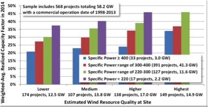
Wind in Australia typically achieves a capacity factor of 30-40%. Ongoing improvements, principally turbine heights, but also blade design, control systems and wind farm design mean that there is reasonable hope that capacity factors can continue to increase. The National Renewable Energy Lab [NREL] explains it thus:
“The lack of an obvious post-2005 trend in average capacity factors can be at least partially explained by two competing influences among more recent project vintages: a continued decline in average specific power (which should boost capacity factors, all else equal) versus a build-out of lower-quality wind resource sites (which should hurt capacity factors, all else equal).
The first of these competing influences—the decline in average “specific power” (i.e., W/m2 of rotor swept area) among more recent turbine vintages—has already been well-documented in Chapter 4 (see, in particular, Figures 24 and 26), but is shown yet again in Figure 33. All else equal, a lower average specific power will boost capacity factors, because there is more swept rotor area available (resulting in greater energy capture) for each watt of rated turbine capacity, meaning that the generator is likely to run closer to or at its rated capacity more often. “
The NREL goes on to show how capacity factors have increased after controlling for wind speed. The image below is taken from a 2014 report: